11 De novo Genome Assembly
For this chapter’s exercises, if not already performed, you will need to download the chapter’s dataset, decompress the archive, and create and activate the conda environment.
Do this, use wget or right click and save to download this Zenodo archive: 10.5281/zenodo.17142958, and unpack
tar xvf denovo-assembly.tar.gz
cd denovo-assembly/
You can then create the subsequently activate environment with
conda env create -f denovo-assembly.yml
conda activate denovo-assemblyThere are additional software requirements for this chapter
Please see the relevant chapter section in Before you start before continuing with this chapter.
11.1 Introduction
First of all, what is a metagenomic sample? Metagenomic sample is a sample that consists of DNA from more than one source. The number and the type of sources might vary widely between different samples. Typical sources for ancient remains are e.g. the host organism and the microbial species. The important part is that we generally do not know the origin of a DNA molecule prior to analysing the sequencing data generated from the DNA library of this sample. In the example presented in Figure 11.1, our metagenomic sample has DNA from three different sources, here coloured in blue, red, and yellow.
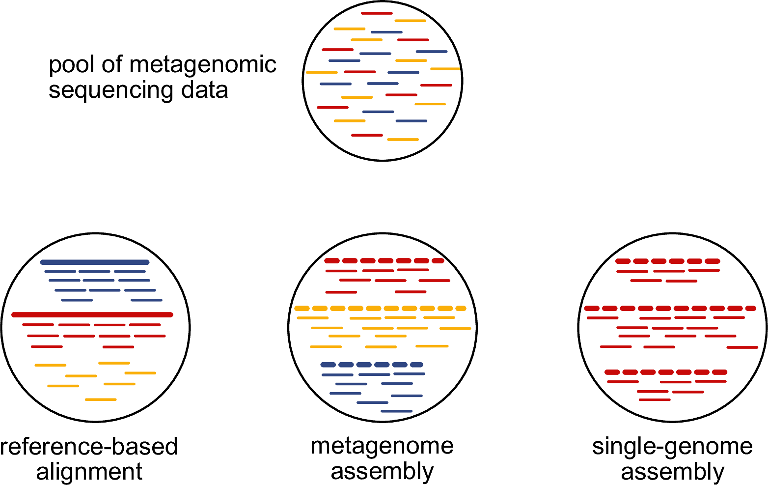
How can we determine the sources of the DNA that we have in our metagenomic sample? There are three main options whose pros and cons are summarised in Table 11.1.
| method | pros | cons |
|---|---|---|
| reference-based alignment | highly sensitive, applicable to aDNA samples | requires all sources to be represented in database |
| single-genome assembly | high-quality genomes from cultivated bacteria | not available for ancient DNA samples |
| metagenome assembly | able to recover unknown diversity present in sample | highly dependent on preservation of ancient DNA |
Until recently, the only option for ancient DNA samples was to take the short-read sequencing data and align them against some known reference genomes. However, this approach is heavily relying on whether all sources of our samples are represented in the available reference genomes. If a source is missing in the reference database - in our toy example, this is the case for the yellow source (Figure 11.1) -, then we will not be able to detect it using this reference database.
While there is a potential workaround for modern metagenomic samples, single-genome assembly relies on being able to cultivate a microbial species to obtain an isolate. This is unfeasible for ancient metagenomic samples because there are no more viable microbial cells available that could be cultivated.
Around 2015, a technical revolution started when the first programs, e.g. MEGAHIT (Li et al. 2015) and metaSPAdes (Nurk et al. 2017), were published that could successfully perform de novo assembly from metagenomic data. Since then, tens of thousands metagenomic samples have been assembled and it was revealed that even well studied environments, such as the human gut microbiome, have a lot of additional microbial diversity that has not been observed previously via culturing and isolation (Almeida et al. 2021).
The technical advancement of being able to perform de novo assembly on metagenomic samples led to an explosion of studies that analysed samples that were considered almost impossible to study beforehand. For researchers that are exposed to ancient DNA, the imminent question arises: can we apply the same methods to ancient DNA data?
In this practical course we will cover how:
- To successfully perform de novo assembly from ancient DNA metagenomic sequencing data
- To reconstruct metagenome-assembled genomes (MAGs) from the assembled contigs
- To validate the quality of the MAGs including determining the presence of ancient DNA damage
11.2 Sample overview
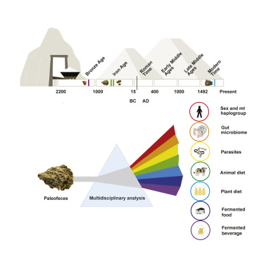
For this practical course, I selected a palaeofaeces sample from the study by Maixner et al. (2021), who generated deep metagenomic sequencing data for four palaeofaeces samples that were excavated from an Austrian salt mine in Hallstatt and were associated with the Celtic Iron Age. We will focus on the youngest sample, 2612, which was dated to be just a few hundred years old (Figure 11.2).
However, because the sample was very deeply sequenced for more than 250 million paired-end reads and we do not want to wait for days for the analysis to finish, we will not use all data but just a sub-sample of them.
You can access the sub-sampled data by making a symbolic link of the chapter pre-made data into the main chapter folder.
ln -s /<PATH>/<TO>/denovo-assembly/seqdata_files/2612_R1.fastq.gz 2612_R1.fastq.gz
ln -s /<PATH>/<TO>/denovo-assembly/seqdata_files/2612_R2.fastq.gz 2612_R2.fastq.gzHow many sequences are in each FastQ file?
Hint: You can run either bioawk.
bioawk -c fastx 'END{print NR}' <FastQ file>or (if installed) you can use seqtk.
seqtk size <FastQ file>to find this out.
There are about 3.25 million paired-end sequences in these files.
11.3 Preparing the sequencing data for de novo assembly
Before running the actual assembly, we need to pre-process our sequencing data. Typical pre-processing steps include the trimming of adapter sequences and barcodes from the sequencing data and the removal of host or contaminant sequences, such as the bacteriophage PhiX, which is commonly sequenced as a quality control.
Many assembly pipelines, such as nf-core/mag, have these steps automatically included, however, these steps can be performed prior to it, too. For this practical course, I have performed these steps for us and we could directly continue with the de novo assembly.
The characteristic of ancient DNA samples that pre-determines the success of the de novo assembly is the distribution of the DNA molecule length. Determine this distribution prior to running the de novo assembly to be able to predict the results of the de novo assembly.
However, since the average length of the insert size of sequencing data (Figure 11.3) is highly correlated with the success of the assembly, we want to first evaluate it. For this we can make use of the program fastp (Chen et al. 2018).

Fastp will try to overlap the two mates of a read pair and, if this is possible, return the length of the merged sequence, which is identical to insert size or the DNA molecule length. If the two mates cannot be overlapped, we will not be able to know the exact DNA molecule length but only know that it is longer than 270 bp (each read has a length of 150 bp and fastp requires a 30 bp overlap between the reads by default).
The final histogram of the insert sizes that is returned by fastp can tell us how well preserved the DNA of an ancient sample is (Figure 11.4). The more the distribution is skewed to the right, i.e. the longer the DNA molecules are, the more likely we are to obtain long contiguous DNA sequences from the de novo assembly. A distribution that is skewed to the left means that the DNA molecules are more highly degraded and this lowers our chances for obtaining long continuous sequences.

To infer the distribution of the DNA molecules, we can run the command
fastp --in1 2612_R1.fastq.gz \
      --in2 2612_R2.fastq.gz \
      --stdout --merge -A -G -Q -L --json /dev/null --html overlaps.html \
> /dev/nullInfer the distribution of the DNA molecule length of the sequencing data. Is this sample well-preserved?
Hint: You can easily inspect the distribution by opening the HTML report overlaps.html in your web browser.
Here is the histogram of the insert sizes determined by fastp (Figure 11.5). By default, fastp will only keep reads that are longer than 30 bp and requires an overlap between the read mates of 30 bp. The maximum read length is 150 bp, therefore, the histogram only spreads from 31 to 271 bp in total.

The sequencing data for the sample 2612 were generated across eight different sequencing runs, which differed in their nominal length. Some sequencing runs were 2x 100 bp, while others were 2x 150 bp. This is the reason why we observe two peaks just short of 100 and 150 bp. The difference to the nominal length is caused by the quality trimming of the data.
Overall, we have almost no short DNA molecules (< 50 bp) but most DNA molecules are longer than 80 bp. Additionally, there were > 200,000 read pairs that could not be overlapped. Therefore, we can conclude that the sample 2612 is moderately degraded ancient DNA sample and has many long DNA molecules.
11.4 De novo assembly
Now, we will actual perform the de novo assembly on the sequencing data. For this, we will use the program MEGAHIT (Li et al. 2015), a de Bruijn-graph assembler.
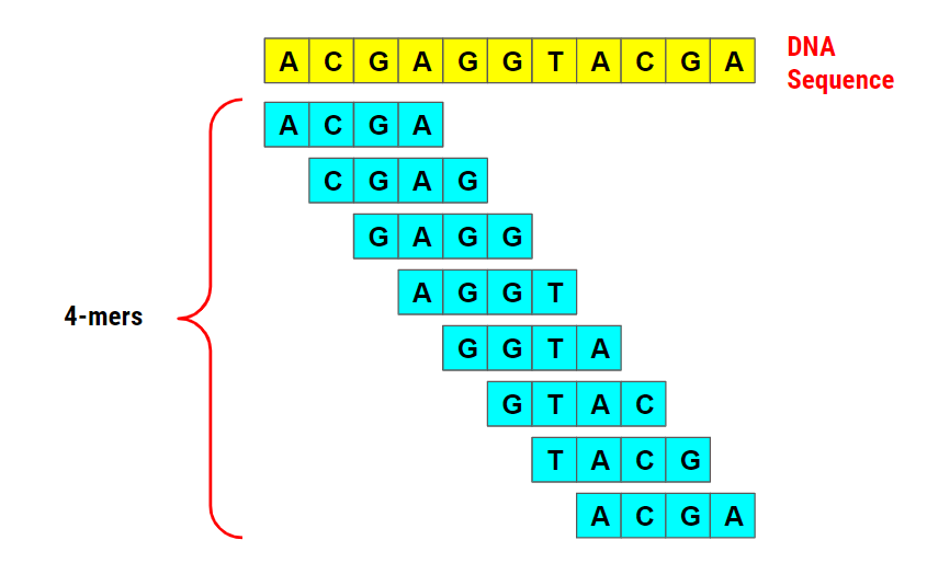
De Bruijn graph assemblers are together with overlap assemblers the predominant group of assemblers. They use k-mers (see Figure 11.6 for an example of 4-mers) extracted from the short-read sequencing data to build the graph. For this, they connect each k-mer to adjacent k-mer using a directional edge. By walking along the edges and visiting each k-mer or node once, longer continuous sequences are reconstructed. This is a very rough explanation and I would advise you to watch this excerpt of a lecture by Rob Edwards from San Diego State University and a Coursera lecture by Ben Langmead from Johns Hopkins University, if you would like to learn more about it.
All de Bruijn graph assemblers work in a similar way so the question is why do we use MEGAHIT and not other programs, such as metaSPAdes?
Pros:
- Low-memory footprint: can be run on computational infrastructure that does not have large memory resources
- It can assembly both single-end and paired-end sequencing data
- The assembly algorithm can cope with the presence of high amounts of ancient DNA damage
Cons:
- It has lower assembly quality on modern comparative data, particularly a higher rate of mis-assemblies (CAMI II challenge)
In the Warinner group, we realised after some tests that MEGAHIT has a clear advantage when ancient DNA damage is present at higher quantities. While it produced a higher number of mis-assemblies compared to metaSPAdes when being evaluated on simulated modern metagenomic data (Critical Assessment of Metagenome Interpretation II challenge, Meyer et al. 2022), it produces more long contigs when ancient DNA damage is present.
To de novo assemble the short-read sequencing data of the sample 2612 using MEGAHIT, we can run the command
megahit -1 2612_R1.fastq.gz \
        -2 2612_R2.fastq.gz \
        -t 14 --min-contig-len 500 \
        --out-dir megahit
This will use the paired-end sequencing data as input and return all contigs that are at least 500 bp long.
While MEGAHIT is able to use merged sequencing data, it is advised to use the unmerged paired-end data as input. In tests using simulated data I have observed that MEGAHIT performed slightly better when using the unmerged data and it likely has something to do with its internal algorithm to infer insert sizes from the paired-end data.
While we are waiting for MEGAHIT to finish, here is a question:
Which k-mer lengths did MEGAHIT select for the de novo assembly?
Based on the maximum read length, MEGAHIT decided to use the k-mer lengths of 21, 29, 39, 59, 79, 99, 119, and 141.
Now, as MEGAHIT has finished, we want to evaluate the quality of the assembly results. MEGAHIT has written the contiguous sequences (contigs) into a single FastA file stored in the folder megahit.
We will process this FastA file with a small script from Heng Li (creator of the famous bwa aligner among others), calN50, which will count the number of contigs and give us an overview of their length distribution.
The script is already present in the chapter’s directory.
k8 ./calN50.js megahit/final.contigs.faHow many contigs were assembled? What is the sum of the lengths of all contigs? What is the maximum, the median, and the minimum contig length?
Hint: The maximum contig length is indicated by the label “N0”, the median by the label “N50”, and the minimum by the label “N100”?
MEGAHIT assembled 3,606 contigs and their lengths sum up to 11.4 Mb. The maximum contig length was 448 kb, the median length was 15.6 kb, and the minimum length was 500 bp.
There is a final caveat when assembling ancient metagenomic data with MEGAHIT: while it is able to assemble sequencing data with a high percentage of C-to-T substitutions, it tends to introduce these changes into the contig sequences, too.
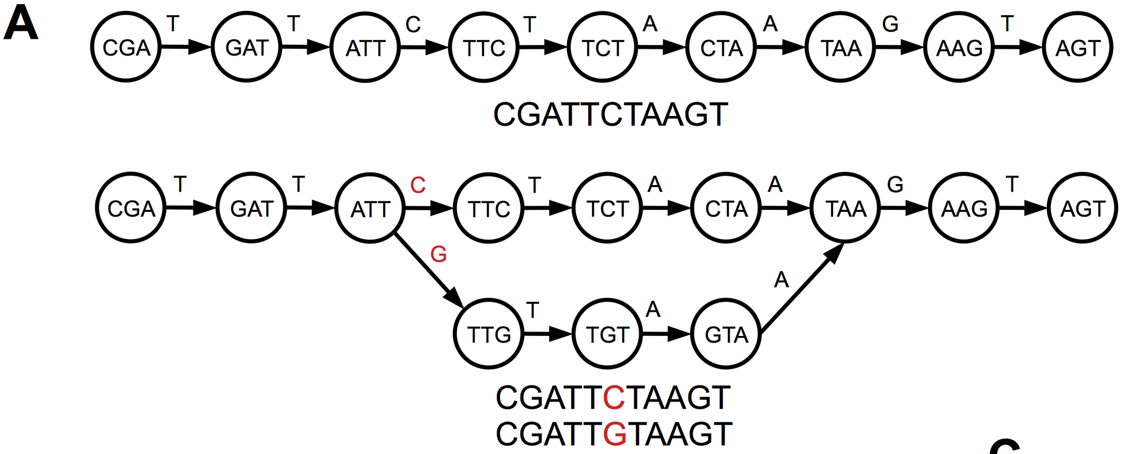
These C-to-T substitutions are similar to biological single-nucleotide polymorphisms in the sequencing data. Both lead the introduction of bubbles in the de Bruijn graph when two alleles are present in the k-mer sequences (Figure 11.7) and the assembler decides during its pruning steps which allele to keep in the contig sequence.
While it does not really matter which allele is kept for biological polymorphisms, it does matter for technical artefacts that are introduced by the presence of ancient DNA damage. In our group we realised that the gene sequences that were annotated on the contigs of MEGAHIT tended to have a higher number of nonsense mutations compared to the known variants of the genes. After manual inspection, we observed that many of these mutations appeared because MEGAHIT chose the damage-derived T allele over the C allele or the damage-derived A allele over a G allele (see Klapper et al. 2023, fig. S1).
To overcome this issue, my colleagues Maxime Borry, James Fellows Yates and I developed a strategy to replace these damage-derived alleles in the contig sequences. This approach consists of aligning the short-read data against the contigs, performing genotyping along them, and finally replacing all alleles for which we have strong support for an allele that is different from the one selected by MEGAHIT.
We standardised this approach and added it to the Nextflow pipeline nf-core/mag (Krakau et al. 2022). It can simply be activated by providing the parameter --ancient_dna.
While MEGAHIT is able to assemble ancient metagenomic sequencing data with high amounts of ancient DNA damage, it tends to introduce damage-derived T and A alleles into the contig sequences instead of the true C and G alleles. This can lead to a higher number of nonsense mutations in coding sequences. We strongly advise you to correct such mutations, e.g. by using the ancient DNA workflow of the Nextflow pipeline nf-core/mag.
11.5 Aligning the short-read data against the contigs
After the assembly, the next detrimental step that is required for many subsequent analyses is the alignment of the short-read sequencing data back to assembled contigs.
Analyses that require these alignment information are for example:
- The correction of the contig sequences to remove damage-derived alleles
- The non-reference binning of contigs into MAGs for inferring the coverage along the contigs
- The quantification of the presence of ancient DNA damage
Aligning the short-read data to the contigs requires multiple steps:
- Build an index from the contigs for the alignment program BowTie2
- Align the short-read data against the contigs using this index with BowTie2
- Calculate the mismatches and deletions of the short-read data against the contig sequences
- Sort the aligned reads by the contig name and the coordinate they were aligned to
- Index the resulting alignment file for faster access
However, these steps are rather time-consuming, even when we just have so little sequencing data as we do for our course example. The alignment is rather slow because we allow a single mismatch in the seeds that are used by the aligner BowTie2 to quickly determine the position of a read along the contig sequences (parameter -N 1). This is necessary because otherwise we might not be able to align reads with ancient DNA damage present on them. Secondly, the larger the resulting alignment file is the longer it takes to sort it by coordinate.
To save us some time and continue with the more interesting analyses, I prepared the resulting files for us. For this, I also corrected damage-derived alleles in the contig sequences. You can access these files on the cluster by running the following commands:
mkdir alignment
ln -s /<PATH>/<TO>/denovo-assembly/seqdata_files/2612.sorted.calmd.bam alignment/
ln -s /<PATH>/<TO>/denovo-assembly/seqdata_files/2612.sorted.calmd.bam.bai alignment/
ln -s /<PATH>/<TO>/denovo-assembly/seqdata_files/2612.fa alignment/
If we wanted to generate the alignments ourselves, we can check the commands in the box below.
To execute the alignment step ourselves we could theoretically run the following commands:
mkdir alignment
ln -s $PWD/megahit/final.contigs.fa alignment/2612.fa
bowtie2-build -f alignment/2612.fa alignment/2612
bowtie2 -p 14 --very-sensitive -N 1 -x alignment/2612 -1 2612_R1.fastq.gz -2 2612_R2.fastq.gz | \
samtools view -Sb - | \
samtools calmd -u /dev/stdin megahit/final.contigs.fa | \
samtools sort -o alignment/2612.sorted.calmd.bam -
samtools index alignment/2612.sorted.calmd.bam
11.6 Reconstructing metagenome-assembled genomes
There are typically two major approaches on how to study biological diversity of samples using the results obtained from the de novo assembly. The first one is to reconstruct metagenome-assembled genomes (MAGs) and to study the species diversity.
“Metagenome-assembled genome” is a convoluted term that means that we reconstructed a genome from metagenomic data via de novo assembly. While these reconstructed genomes, particularly the high-quality ones, are most likely a good representation of the genomes of the organisms present in the sample, the scientific community refrains from calling them a species or a strain. The reason is that for calling a genome a species or a strain additional analyses would be necessary, of which many would include the cultivation of the organism. For many samples, this is not feasible and therefore the community stuck to the term MAG instead.
The most commonly applied method to obtain MAGs is the so-called “non-reference binning”. Non-reference binning means that we do not try to identify contigs by aligning them against known reference genomes, but only use the characteristics of the contigs themselves to cluster them (Figure 11.8).
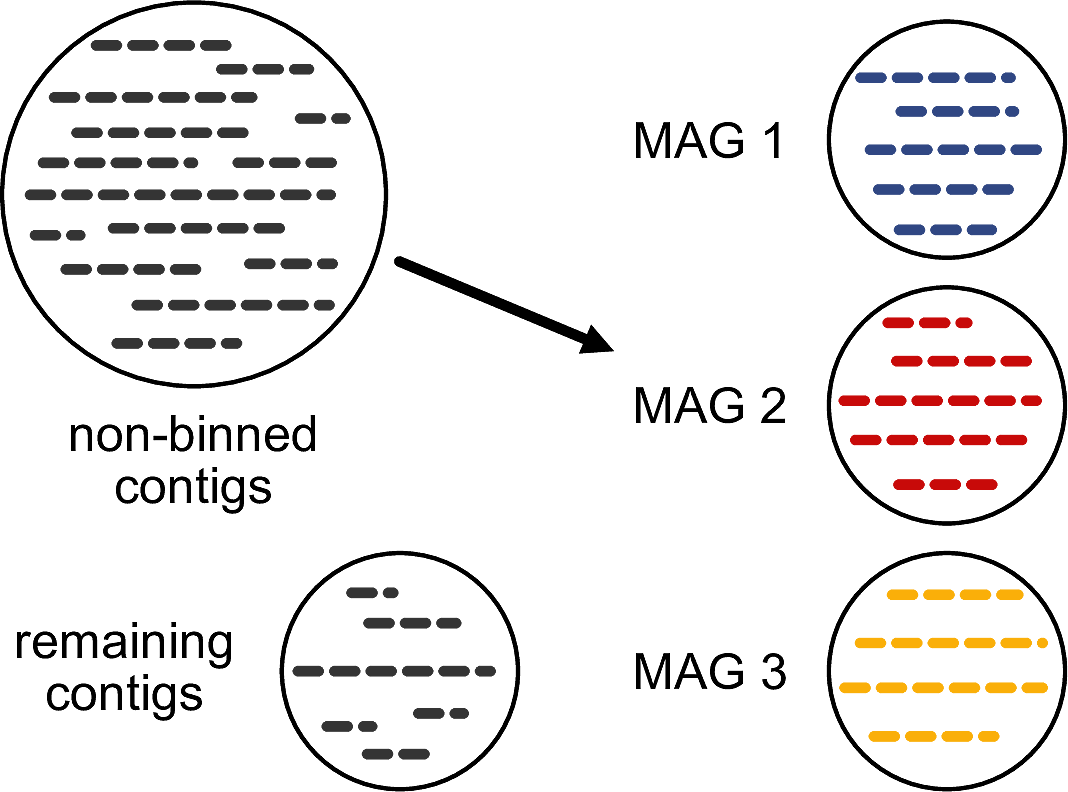
The two most commonly used characteristics are:
- The tetra-nucleotide frequency: the frequency of all 4-mers (e.g. AAAA, AAAC, AAAG etc.) in the contig sequence
- The coverage along the contig
The idea here is that two contigs that are derived from the same bacterial genome will likely have a similar nucleotide composition and coverage.
This approach works very well when the contigs are longer and they strongly differ in the nucleotide composition and the coverage from each other. However, if this is not the case, e.g. there is more than one strain of the same species in the sample, these approaches will likely not be able to assign some contigs to clusters: these contigs remain unbinned. In case there is a high number of unbinned contigs, one can also employ the more sensitive reference-based binning strategies but we will not cover this in this practical course.
There are a number of different binning tools out there that can be used for this task. Since this number is constantly growing, there have been attempts to standardise the test data sets that these tools are run on so that their performances can be easily compared. The most well-known attempt is the Critical Assessment of Metagenome Interpretation (Critical Assessment of Metagenome Interpretation II challenge, Meyer et al. 2022), which released the latest comparison of commonly used tools for assembly, binning, and bin refinement in 2022. I recommend that you first check the performance of a new tool against the CAMI datasets before testing it to see whether it is worth using it.
Three commonly used binners are:
- metaBAT2 (Kang et al. 2019, more than 2,000 citations)
- MaxBin2 (Wu, Simmons, and Singer 2016, more than 1,700 citations)
- CONCOCT (Alneberg et al. 2014, more than 1,800 citation)
Each of these three binners employs a slightly different strategy. While metaBAT2 simply uses the two previously mentioned metrics, the tetra-nucleotide frequency and the coverage along the contigs, MaxBin2 additionally uses single-copy marker genes to infer the taxonomic origin of contigs. In contrast, CONCOCT also just uses the two aforementioned metrics but first performs a Principal Component Analysis (PCA) on these metrics and uses the PCA results for the clustering.
The easiest way to run all these three programs is the program metaWRAP (Uritskiy, DiRuggiero, and Taylor 2018). metaWRAP is in fact a pipeline that allows you to assemble your contigs, bin them, and subsequently refine the resulting MAGs. However, the pipeline is not very well written and does not contain any strategies to deal with ancient metagenomic sequencing data. Therefore, I prefer to use different pipelines, such as nf-core/mag for the assembly, and only use metaWRAP for binning and bin refinement.
Make sure you have followed the instructions for setting up the additional software requirements for this chapter already! See the beginning of the chapter for more information.
To skip the first steps of metaWRAP and start straight with the binning, we need to create the folder structure and files that metaWRAP expects:
mkdir -p metawrap/INITIAL_BINNING/2612/work_files
ln -s $PWD/alignment/2612.sorted.calmd.bam \
    metawrap/INITIAL_BINNING/2612/work_files/2612.bam
mkdir -p metawrap/faux_reads
echo "@" > metawrap/faux_reads/2612_1.fastq
echo "@" > metawrap/faux_reads/2612_2.fastq
Now, we can start to run the binning. In this practical course, we will focus on metaBAT2 and MaxBin2. To bin the contigs with these binners, we execute:
conda activate metawrap-env
metawrap binning -o metawrap/INITIAL_BINNING/2612 \
    -t 14 \
    -a alignment/2612.fa \
    --metabat2 --maxbin2 --universal \
metawrap/faux_reads/2612_1.fastq metawrap/faux_reads/2612_2.fastqMetaWRAP is not a well-written Python software and has not been update for more than three years. It still relies on the deprecated Python v2.7. This is in conflict with many other tools and therefore it requires its own conda environment, metawrap-env. Do not forget to deactivate this environment afterwards again!
MetaWRAP will run metaBAT2 and MaxBin2 for us and store their respective output into sub-folders in the folder metawrap/INITIAL_BINNING/2612.
How many bins did metaBAT2 and MaxBin2 reconstruct, respectively? Is there a difference in the genome sizes of these reconstructed bins?
Hint: You can use the previously introduced script k8 ./calN50.js to analyse the genome size of the individual bins.
metaBAT2 reconstructed seven bins, while MaxBin2 reconstructed only five bins.
When comparing the genome sizes of these bins, we can see that despite having reconstructed fewer bins, MaxBin2’s bins have on average larger genome size and all of them are at least 1.5 Mb. In contrast, five out of seven metaBAT2 bins are shorter than 1.5 Mb.
While we could have run these two binning softwares manually ourselves, there is another reason why we should use metaWRAP: it has a powerful bin refinement algorithm.
As we just observed, binning tools come to different results when performing non-reference binning on the same contigs. So how do we know which binning tool delivered the better or even correct results?
A standard approach is to identify single-copy marker genes that are specific for certain taxonomic lineages, e.g. to all members of the family Prevotellaceae or to all members of the kingdom archaea. If we find lineage-specific marker genes from more than one lineage in our bin, something likely went wrong. While in certain cases horizontal gene transfer could explain such a finding, it is much more common that a binning tool clustered two contigs from two different taxons.
During its bin refinement, metaWRAP first combines the results of all binning tools in all combinations. So it would merge the results of metaBAT2 and MaxBin2, metaBAT2 and CONCOCT, MaxBin2 and CONCOCT, and all three together. Afterwards, it evaluates the presence of lineage-specific marker genes on the contigs of the bins for every combination and the individual binning tools themselves. In the case that it would find marker genes of more than one lineage in a bin, it would split the bin into two. After having evaluated everything, metaWRAP selects the refined bins that have the highest quality score across the whole set of bins.

Using this approach, the authors of metaWRAP could show that they can outperform the individual binning tools and other bin refinement algorithms both regarding the completeness and contamination that was estimated for the MAGs (Figure 11.9).
Due to the large memory requirements of the the bin refinment module, we have prepared the results of metaWRAP’s bin refinement algorithm, metawrap_50_10_bins.stats for you already, which can be found in the folder /<PATH>/<TO>/denovo-assembly/seqdata_files.
Running metaWRAP’s bin refinement module requires about 72 GB of memory because it has to load a larger reference database containing the lineage-specific marker genes of checkM.
If you have sufficient computational memory resources, you can run the following steps to run the bin refinement yourself.
To apply metaWRAP’s bin refinement to the bins that we obtained from metaBAT2 and MaxBin2, we first need to install the software checkM (Parks et al. 2015) that will provide the lineage-specific marker gene catalogue:
## Only run if you have at least 72 GB of memory!
mkdir checkM
wget -O checkM/checkm_data_2015_01_16.tar.gz \
    https://data.ace.uq.edu.au/public/CheckM_databases/checkm_data_2015_01_16.tar.gz
tar xvf checkM/checkm_data_2015_01_16.tar.gz -C checkM

echo checkM | checkm data setRoot checkM
Afterwards, we can execute metaWRAP’s bin refinement module:
## Only run if you have at least 72 GB of memory!
mkdir -p metawrap/BIN_REFINEMENT/2612
metawrap bin_refinement -o metawrap/BIN_REFINEMENT/2612 \
    -t 14 \
    -c 50 \
    -x 10 \
    -A metawrap/INITIAL_BINNING/2612/maxbin2_bins \
    -B metawrap/INITIAL_BINNING/2612/metabat2_bins
Once finished you can deactivate the metawrap conda environment.
conda deactivateThe latter step will produce a summary file, metawrap_50_10_bins.stats, that lists all retained bins and some key characteristics, such as the genome size, the completeness estimate, and the contamination estimate. The latter two can be used to assign a quality score according to the Minimum Information for MAG (MIMAG; see info box).
The two most common metrics to evaluate the quality of MAGs are:
- The completeness: how many of the expected lineage-specific single-copy marker genes were present in the MAG?
- The contamination: how many of the expected lineage-specific single-copy marker genes were present more than once in the MAG?
These metric is usually calculated using the marker-gene catalogue of checkM (Parks et al. 2015), also if there are other estimates from other tools such as BUSCO (Manni et al. 2021), GUNC (Orakov et al. 2021) or checkM2 (Chklovski et al. 2022).
Depending on the estimates on completeness and contamination plus the presence of RNA genes, MAGs are assigned to the quality category following the Minimum Information for MAG criteria (Bowers et al. 2017). You can find the overview here.
As these two steps will run rather long and need a large amount of memory and disk space, I have provided the results of metaWRAP’s bin refinement. You can find the file here: /<PATH>/<TO>/denovo-assembly/metawrap_50_10_bins.stats. Be aware that these results are based on the bin refinement of the results of three binning tools and include CONCOCT.
How many bins were retained after the refinement with metaWRAP? How many high-quality and medium-quality MAGs did the refinement yield following the MIMAG criteria?
Hint: You can more easily visualise tables on the terminal using the Python program visidata. You can open a table using vd -f tsv /<PATH>/<TO>/denovo-assembly/metawrap_50_10_bins.stats. (press ctrl + q to exit). Next to separating the columns nicely, it allows you to perform a lot of operations like sorting conveniently. Check the cheat sheet here.
In total, metaWRAP retained five bins, similarly to MaxBin2. Of these five bins, the bins bin.3 and bin.4 had completeness and contamination estimates that would qualify them for being high-quality MAGs. However, we would need to check the presence of rRNA and tRNA genes. The other three bins are medium-quality bins because their completeness estimate was < 90%.
11.7 Taxonomic assignment of contigs
What should we do when we simply want to know to which taxon a certain contig most likely belongs to?
Reconstructing metagenome-assembled genomes requires multiple steps and might not even provide the answer in the case that the contig of interest is not binned into a MAG. Instead, it is sufficient to perform a sequence search against a reference database.
There are plenty of tools available for this task, such as:
- BLAST/DIAMOND
- Kraken2
- Centrifuge
- MMSeqs2
For each tool, we can either use pre-computed reference databases or compute our own one. The two taxonomic classification systems that are most commonly used are:
- NCBI Taxonomy
- GTDB
As for any task that involves the alignment of sequences against a reference database, the chosen reference database should fit the sequences you are searching for. If your reference database does not capture the diversity of your samples, you will not be able to assign a subset of the contigs. There is also a trade-off between a large reference database that contains all sequences and its memory requirement. Wright, Comeau, and Langille (2023) elaborated on this quite extensively when comparing Kraken2 against MetaPhlAn.
While all of these tools can do the job, I typically prefer to use the program MMSeqs2 (Steinegger and Söding 2017) because it comes along with a very fast algorithm based on amino acid sequence alignment and implements a lowest common ancestor (LCA) algorithm (Figure 11.10). Recently, they implemented a taxonomy workflow (Mirdita et al. 2021) that allows to efficiently assign contigs to taxons. Luckily, it comes with multiple pre-computed reference databases, such as the GTDB v214 reference database (Parks et al. 2020), and therefore it is even more accessible for users.
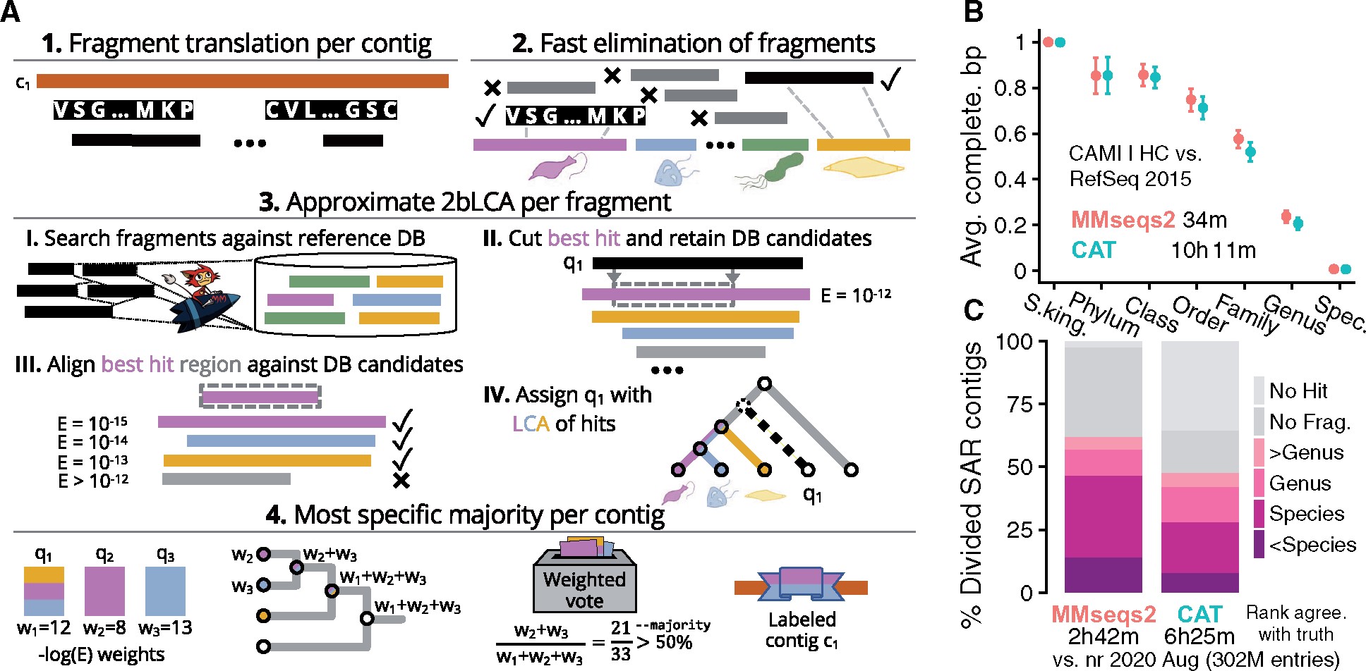
The latest version of the pre-computed GTDB reference database (r214) requires about 132 GB of harddisk space and 850 GB of memory for running.
Therefore for those on smaller computational infrastructure, I have pre-computed the results. You can find the results 2612.mmseqs2_gtdb.tsv in the folder /<PATH>/<TO>/denovo-assembly/seqdata_files. These results are based on the slightly older GTDB reference database r207.
An alternative for users with a less powerful infrastructure is the program KrakenUniq, however if your infrastructure has sufficient computational resources, or you want to see how you would run mmseqs2 see the collapsed block.
Before running MMSeqs2’s taxonomy workflow against the GTDB reference database, we need to install it.
## Only run if you have at least 105 GB of disk space!
mkdir -p refdbs/mmseqs2/gtdb
mmseqs databases GTDB \
    refdbs/mmseqs2/gtdb /tmp --threads 14
Subsequently, we can align all the contigs of the sample 2612 against the GTDB r207 with MMSeqs2:
## Only run if you have at least 700 GB of memory!
mkdir mmseqs2
mmseqs createdb alignment/2612.fa mmseqs2/2612.contigs
mmseqs taxonomy  mmseqs2/2612.contigs \
    refdbs/mmseqs2/gtdb/mmseqs2_gtdb \
    mmseqs2/2612.mmseqs2_gtdb \
    /tmp \
    -a --tax-lineage 1 \
    --lca-ranks kingdom,phylum,class,order,family,genus,species \
    --orf-filter 1 \
    --remove-tmp-files 1 \
    --threads 14
mmseqs createtsv mmseqs2/2612.contigs \
    mmseqs2/2612.mmseqs2_gtdb \
Lets inspect the file 2612.mmseqs2_gtdb.tsv in the folder /<PATH>/<TO>/denovo-assembly/seqdata_files.
What is the proportion of contigs that could be assigned to the different taxonomic ranks, such as species or genus? What are the dominant taxa?
Hint: You can access this information easily by opening the file using visidata: vd seqdata/2612.mmseqs2_gtdb.tsv (press ctrl + q to exit)
From the 3,606 contigs, MMSeqs2’s taxonomy workflow assigned 3,523 contigs to any taxonomy. For the rest, there was not enough information and they were discarded.
From the 3,523 assigned contigs, 2,013 were assigned to the rank “species”, while 1,137 could only be assigned to the rank “genus”.
The most contigs were assigned the archael species Halococcus morrhuae (n=386), followed by the bacterial species Olsenella E sp003150175 (n=298) and Collinsella sp900768795 (n=186).
11.8 Taxonomic assignment of MAGs
MMSeqs2’s taxonomy workflow is very useful to classify all contigs taxonomically. However, how would we determine which species we reconstructed by binning our contigs?
The simplest approach would be that we could summarise MMSeqs2’s taxonomic assignments of all contigs of a MAG and then determine which lineage is the most frequent one. Although this would work in general, there is another approach that is more sophisticated: GTDB toolkit (GTDBTK, Chaumeil et al. 2020).
GTDBTK performs three steps to assign a MAG to a taxonomic lineage:
- Lineage identification based on single-copy marker genes using Hidden Markov Models (HMMs)
- Multi-sequence alignment of the identified marker genes
- Placement of the MAG genome into a fixed reference tree at class level
The last step is particularly clever. Based on the known diversity of a lineage present in the GTDB, it will construct a reference tree with all known taxa of this lineage. Afterwards, the tree structure is fixed and an algorithm attempts to create a new branch in the tree for placing the unknown MAG based on both the tree structure and the multi-sequence alignment.
In most cases, both the simple approach of taking the majority of the MMSeqs2’s taxonomy results and the GTDBTK approach lead to very similar results. However, GTDBTK performs better when determining whether a new MAG potentially belongs to a new genus or even a new family.
To infer which taxa our five reconstructed MAGs represent, we can run the GTDBTK.
The latest version of the database used by GTDBTK (r214) requires about 83 GB of harddisk space and 80 GB of memory for running.
Therefore for those on smaller computational infrastructure, I have pre-computed the results with the slightly older version of GTDBTK (r207). You can find the results 2612.gtdbtk_archaea.tsv and 2612.gtdbtk_bacteria.tsv in the folder /<PATH>/<TO>/denovo-assembly/seqdata_files.
If you want to see how you would run the gtdbtk classify_wf see the collapsed block.
First, we need to install the GTDB database:
## Only run if you have at least 70 GB disk space!
mkdir -p refdbs/gtdbtk
wget -O refdbs/gtdbtk/gtdbtk_v2_data.tar.gz \
    https://data.gtdb.ecogenomic.org/releases/latest/auxillary_files/gtdbtk_v2_data.tar.gz
tar xvf refdbs/gtdbtk/gtdbtk_v2_data.tar.gz -C refdbs/gtdbtk
Afterwards, we can run GTDBTK’s classify workflow:
## Only run if you have at least 80 GB of memory!
mkdir gtdbtk
GTDBTK_DATA_PATH="$PWD/refdbs/gtdbtk/gtdbtk_r207_v2" \
gtdbtk classify_wf --cpu 14 --extension fa \
    --genome_dir metawrap/BIN_REFINEMENT/2612/metawrap_50_10_bins \
    --out_dir gtdbtk
Lets inspect files 2612.gtdbtk_archaea.tsv and 2612.gtdbtk_bacteria.tsv in the folder /<PATH>/<TO>/denovo-assembly/seqdata_files.
Do the classifications obtained by GTDBTK match the classifications that were assigned to the contigs using MMSeqs2? Would you expect these taxa given the archaeological context of the samples?
Hint: You can access the classification results of GTDBTK easily by opening the file using visidata: vd 2612.gtdbtk_archaea.tsv and vd 2612.gtdbtk_bacteria.tsv (press ctrl + q to exit)
The five MAGs reconstructed from the sample 2612 were assigned to the taxa:
bin.1: Agathobacter rectalisbin.2: Halococcus morrhuaebin.3: Methanobrevibacter smithiibin.4: Ruminococcus bromiibin.5: Bifidobacterium longum
All of these species were among the most frequent lineages that were identified by MMSeqs2’s taxonomy workflow highlighting the large overlap between the methods.
We would expect all five species to be present in our sample. All MAGs but bin.2 were assigned to human gut microbiome commensal species that are typically found in healthy humans. The MAG bin.2 was assigned to a halophilic archaeal species, which is typically found in salt mines.
11.9 Evaluating the amount of ancient DNA damage
One of the common questions that remain at this point of our analysis is whether the contigs that we assembled show evidence for the presence of ancient DNA damage. If yes, we could argue that these microbes are indeed ancient, particularly when their DNA fragment length distribution is rather short, too.
MAGs typically consist of either tens or hundreds of contigs. For this case, many of the commonly used tools for quantifying the amount of ancient DNA damage, such as damageprofiler (Neukamm, Peltzer, and Nieselt 2021) or mapDamage2 (Jónsson et al. 2013), are not very well suited because they would require us to manually check each of their generated “smiley plots”, which visualise the amount of C-to-T substitutions at the end of reads.
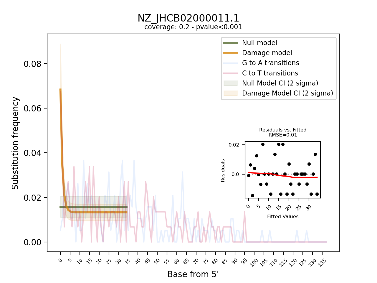
Instead, we will use the program pyDamage (Borry et al. 2021) that was written with the particular use-case of metagenome-assembled contigs in mind. Although pyDamage can visualise the amount of C-to-T substitutions at the 5’ end of reads, it goes a step further and fits two models upon the substitution frequency (Figure 11.11). The null hypothesis is that the observed distribution of C-to-T substitutions at the 5’ end of reads reflects a flat line, i.e. a case when no ancient DNA damage is present. The alternative model assumes that the distribution resembles an exponential decay, i.e. a case when ancient DNA damage is present. By comparing the fit of these two models to the observed data for each contig, pyDamage can quickly identify contigs that are likely of ancient origin without requiring the user to inspect the plots visually.
We can run pyDamage directly on the alignment data in BAM format:
pydamage analyze -w 30 -p 14 alignment/2612.sorted.calmd.bamEvaluate the pyDamage results with respect to the amount of C-to-T substitutions observed on the contigs! How many contigs does pyDamage consider to show evidence for ancient DNA damage? How much power (prediction accuracy) does it have for this decision? Which MAGs are strongly “ancient” or “modern”?
Hint: You can access pyDamage’s results easily by opening the file using visidata: vd pydamage_results/pydamage_results.csv (press ctrl + q to exit)
From the 3,606 contigs, pyDamage inferred a q-value, i.e. a p-value corrected for multiple testing, of < 0.5 to 26 contigs. This is partially due to a high fraction of the contigs with no sufficient information to discriminate between the models (predicted accuracy of < 0.5). However, the majority of the contigs with a prediction accuracy of > 0.5 still had q-values of 0.05 and higher. This suggests that overall the sample did not show large evidence of ancient DNA damage.
This reflects also on the MAGs. Although four of the five MAGs were human gut microbiome taxa, they did not show strong evidence of ancient DNA damage. This suggests that the sample is too young and is well preserved.
11.10 Annotating genomes for function
The second approach on how to study biological diversity of samples using the assembly results is to compare the reconstructed genes and their functions with each other.
While it is very interesting to reconstruct the metagenome-assembled genomes from contigs and speculate about the evolution of a certain taxon, this does not always help when studying the ecology of a microbiome. Studying the ecology of a microbiome means to understand which taxa are present in an environment, what type of community do they form, what kind of natural products do they produce etc.?
With the lack of any data from culture isolates, it is rather difficult to discriminate from which species a reconstructed gene sequence is coming from, particularly when the contigs are short. Many microbial species exchange genes among each other via horizontal gene transfer which leads to multiple copies of a gene to be present in our metagenome and increases the level of difficulty further.
Because of this, many researchers tend to annotate all genes of a MAGs and compare the presence and absence of these genes across other genomes that were taxonomically assigned to the same taxon. This analysis, called pan-genome analysis, allows us to estimate the diversity of a microbial species with respect to their repertoire of protein-coding genes.
One of the most commonly used annotation tools for MAGs is Prokka (Seemann 2014), although it has recently been challenged by Bakta (Schwengers et al. 2021). The latter provides the same functionality as Prokka but incorporates more up-to-date reference databases for the annotation. Therefore, the scientific community is slowly shifting to Bakta.
Next to returning information on the protein-coding genes, Prokka also returns the annotation of RNA genes (tRNAs and rRNAs), which will help us to evaluate the quality of MAGs regarding the MIMAG criteria.
For this practical course, we will use Prokka and we will focus on annotating the pre-refined MAG bin bin.3.fa that we reconstructed from the sample 2612.
prokka --outdir prokka \
    --prefix 2612_003 \
    --compliant --metagenome --cpus 14 \
seqdata_files/metawrap_50_10_bins/bin.3.faIf you performed your own metaWRAP bin refineent, you would find the bin.3.fa in the metawrap/BIN_REFINEMENT directory.
Prokka has annotated our MAG. What type of files does Prokka return? How many genes/tRNAs/rRNAs were detected?
Hint: Check the file prokka/2612_003.txt for the number of annotated elements.
Prokka returns the following files:
.faa: the amino acid sequences of all identified coding sequences.ffn: the nucleotide sequences of all identified coding sequences.fna: all contigs in nucleotide sequence format renamed following Prokka’s naming scheme.gbk: all annotations and sequences in GenBank format.gff: all annotations and sequences in GFF format.tsv: the tabular overview of all annotations.txt: the short summary of the annotation results
Prokka found 1,797 coding sequences, 32 tRNAs, but no rRNAs. Finding no rRNAs is a common issues when trying to assemble MAGs without long-read sequencing data and is not just characteristic for ancient DNA samples. However, this means that we cannot technically call this MAG a high-quality MAG due to the lack of the rRNA genes.
11.11 (Optional) clean-up
If you plan to run through the ancient metagenomic pipelines chapter, do not clear up the denovo assembly directory yet! The data from this chapter will be re-used.
Let’s clean up your working directory by removing all the data and output from this chapter.
The command below will remove the /<PATH>/<TO>/denovo-assembly directory as well as all of its contents.
Always be VERY careful when using rm -r. Check 3x that the path you are specifying is exactly what you want to delete and nothing more before pressing ENTER!
rm -rf /<PATH>/<TO>/denovo-assembly*Once deleted you can move elsewhere (e.g. cd ~).
We can also get out of the conda environment with
conda deactivateTo delete the conda environment
conda remove --name denovo-assembly --all -y11.12 Summary
In this practical course you have gone through all the important steps that are necessary for de novo assembling ancient metagenomic sequencing data to obtain contiguous DNA sequences with little error. Furthermore, you have learned how to cluster these sequences into bins without using any references and how to refine them based on lineage-specific marker genes. For these refined bins, you have evaluated their quality regarding common standards set by the scientific community and assigned the MAGs to its most likely taxon. Finally, we learned how to infer the presence of ancient DNA damage and annotate them for RNA genes and protein-coding sequences.
Be aware of the sequencing depth when you assemble your sample. This sample used in this practical course was not obtained by randomly subsampling but I subsampled the sample so that we are able to reconstruct MAGs.
The original sample had almost 200 million reads, however, I subsampled it to less than 5 million reads. You usually need a lot of sequencing data for de novo assembly and definitely more data than for reference-alignment based profiling. However, it also heavily depends on the complexity of the sample. So the best advice is: just give it a try!